Computing Multiple Transport Coefficients

Note

Referencing this data structure directly corresponds to the entries in each of the input arrays. For example, if you wish to print the self-diffusion coefficient from the above code block for carbon (0th element of the Z array), at 10 g/cc (1st element of the rho_i array), at 0.4 eV (2nd element of the T array), you would use the syntax print(D[1,2,0]) (marked in red in Fig. 1).

import numpy as np
import matplotlib.pyplot as plt

from plasma_properties import transport


Am = np.array([1.9944235e-23, 4.4803895e-23, 8.4590343e-23]) # Atomic masses for each element [g]
rho_i = np.array([1,10,100]) # Mass densities [g/cc]
T = np.arange(0.2, 200, 0.1) # Temperature range [eV]
Z = np.array([6, 13, 23]) # Nuclear charge for each element

# Instantiate the Stanton-Murillo transport submodule
sm = transport.SM(Am, rho_i, T, Z, units_out='cgs')

# Compute transport
D = sm.self_diffusion()
eta = sm.viscosity()
K = sm.thermal_conductivity()


fig, ax = plt.subplots(1, 3, figsize=(30,8))

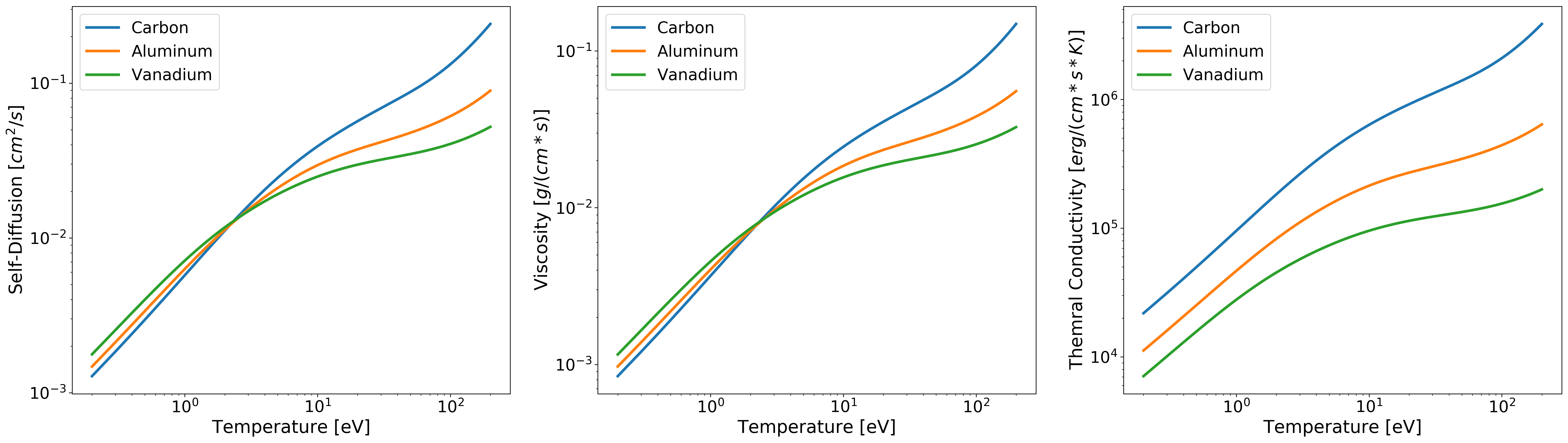
#---------------- Plotting Self-Diffusion ----------------#
ax[0].loglog(T, D[0,:,0], linewidth=3, label='Carbon')
ax[0].loglog(T, D[0,:,1], linewidth=3, label='Aluminum')
ax[0].loglog(T, D[0,:,2], linewidth=3, label='Vanadium')

ax[0].set_xlabel('Temperature [eV]', fontsize=20)
ax[0].set_ylabel('Self-Diffusion $[cm^2/s]$', fontsize=20)
ax[0].tick_params(axis="x", labelsize=18)
ax[0].tick_params(axis="y", labelsize=18)

#------------------ Plotting Viscosity -------------------#
ax[1].loglog(T, eta[0,:,0], linewidth=3, label='Carbon')
ax[1].loglog(T, eta[0,:,1], linewidth=3, label='Aluminum')
ax[1].loglog(T, eta[0,:,2], linewidth=3, label='Vanadium')

ax[1].set_xlabel('Temperature [eV]', fontsize=20)
ax[1].set_ylabel('Viscosity $[g/(cm * s)]$', fontsize=20)
ax[1].tick_params(axis="x", labelsize=18)
ax[1].tick_params(axis="y", labelsize=18)


#-------------- Plotting Thermal Conductivity ------------#
ax[2].loglog(T, K[0,:,0], linewidth=3, label='Carbon')
ax[2].loglog(T, K[0,:,1], linewidth=3, label='Aluminum')
ax[2].loglog(T, K[0,:,2], linewidth=3, label='Vanadium')

ax[2].set_xlabel('Temperature [eV]', fontsize=20)
ax[2].set_ylabel('Thermal Conductivity $[erg/(cm * s * K)]$', fontsize=20)
ax[2].tick_params(axis="x", labelsize=18)
ax[2].tick_params(axis="y", labelsize=18)

plt.legend(fontsize=18)
plt.show()