User’s Guide
The Transport Module
Currently, the plasma_properties package allows users to compute single a transport coefficient or across a range of elements, mass densities, and temperatures using the Stanton and Murillo model. Refer to Fig 1. for the structure of the output in the multi-element/mass-density/temperature case.
The current capabilities include computing a single transport coefficient for a given atomic mass [g], nuclear charge (atomic number), temperature [eV], and mass density [g/cc].
Note
The atomic mass and atomic number are coupled. When computing transport for a range of elements and isotopes, the entry in each array must correspond.
For example, if you wanted to compute transport coefficients for three isotopes of hydrogen and one isotope of helium, the input arrays would be structured as follows:
# Atomic mass for each isotope [1H, 2H, 3H, 1He] in grams
Am = np.array([1.6735e-24, 3.3445e-24, 5.0083e-24, 6.6464e-24])

# Nuclear charge for hydrogen and each of its isotopes and helium [1H, 2H, 3H, 1He]
Z = np.array([1, 1, 1, 2])
Computing a Single Transport Coefficient
To compute a single transport coefficient do the following:
from plasma_properties import transport

Am = 1.9944235e-23 # Atomic mass of element [g]
rho_i = 1 # Mass density [g/cc]
T = 0.2 # Temperature [eV]
Z = 6 # Nuclear charge for carbon

# Instantiate the Stanton-Murillo transport submodule
sm = transport.SM(Am, rho_i, T, Z, units_out='cgs')

# Compute transport coefficients
D = sm.self_diffusion()
eta = sm.viscosity()
K = sm.thermal_conductivity()

print(D, eta, K)
Output (in cgs units):
[0.00127858] [0.00084193] [21856.10137931]
Computing Multiple Transport Coefficients
Computing transport coefficients for a range of elements, mass densities, and temperatures follows
the same syntax as the single transport case except the inputs are now numpy.array().
Below is example input for this case:
import numpy as np
from plasma_properties import transport

Am = np.array([1.9944235e-23, 4.4803895e-23, 8.4590343e-23]) # Atomic masses for each element [g]
rho_i = np.array([1,10,100]) # Mass densities [g/cc]
T = np.arange(0.2, 200, 0.1) # Temperature range [eV]
Z = np.array([6, 13, 23]) # Nuclear charge for each element

# Instantiate the Stanton-Murillo transport submodule
sm = transport.SM(Am, rho_i, T, Z, units_out='cgs')

# Compute transport
D = sm.self_diffusion()
eta = sm.viscosity()
K = sm.thermal_conductivity()
The output of the above code will be a 3-dimensional numpy.ndarray() where the axes have the following structure.
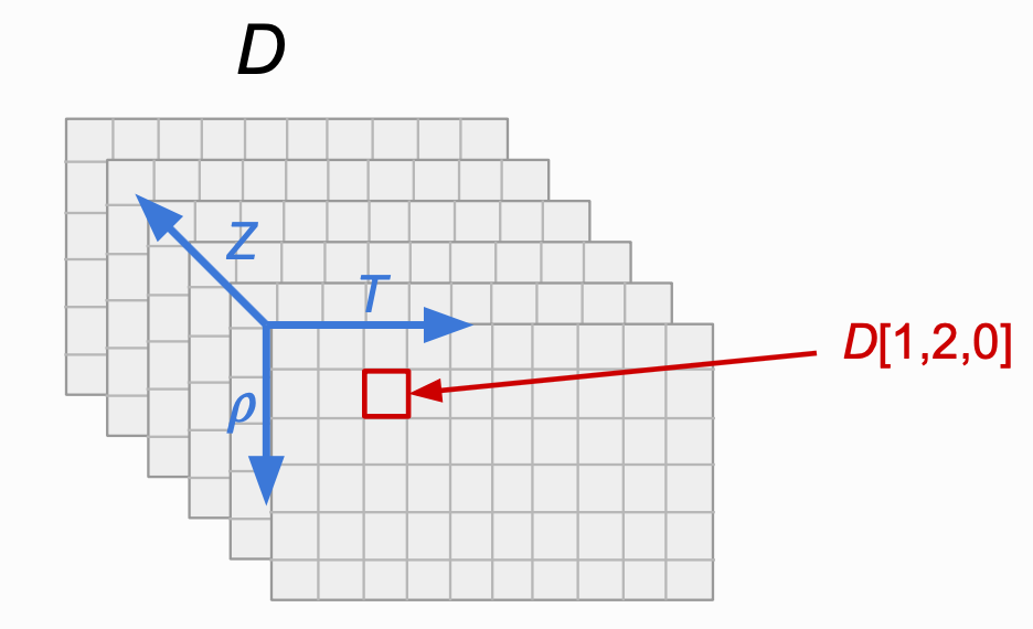
Fig 1. The shape of the data structure that is output for the case of multi-element/temperature/density transport coefficients. Note that each 2-dimensional “slice” in the Z direction corresponds to a different element, and moving along the positive \(\rho\)/T direction corresponds to an increase in the mass-density/temperature for a fixed element.
Note
Referencing this data structure directly corresponds to the entries in each of the input arrays. For example, if you wish to print the self-diffusion coefficient from the above code block for carbon (0th element of the Z array), at 10 g/cc (1st element of the rho_i array), at 0.4 eV (2nd element of the T array), you would use the syntax
print(D[1,2,0]) (marked in red in Fig. 1).
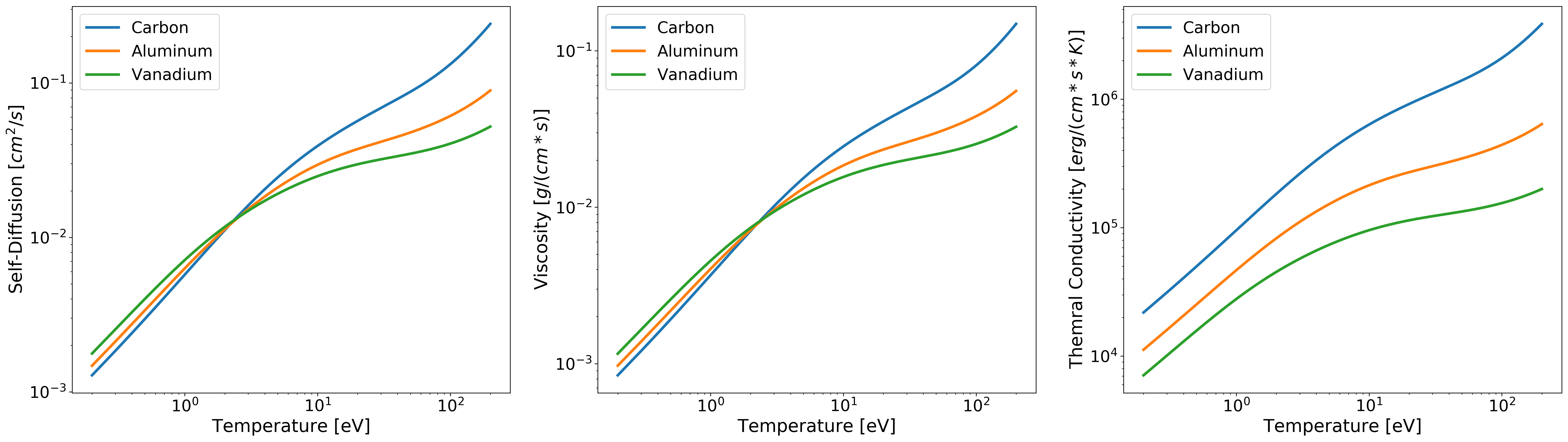
Below is some example code for plotting data the data produce in the multiple element/mass-density/temperature case from the code block above:
import matplotlib.pyplot as plt

fig, ax = plt.subplots(1, 3, figsize=(30,8))

#---------------- Plotting Self-Diffusion ----------------#
ax[0].loglog(T, D[0,:,0], linewidth=3, label='Carbon')
ax[0].loglog(T, D[0,:,1], linewidth=3, label='Aluminum')
ax[0].loglog(T, D[0,:,2], linewidth=3, label='Vanadium')

ax[0].set_xlabel('Temperature [eV]', fontsize=20)
ax[0].set_ylabel('Self-Diffusion $[cm^2/s]$', fontsize=20)
ax[0].tick_params(axis="x", labelsize=18)
ax[0].tick_params(axis="y", labelsize=18)

#------------------ Plotting Viscosity -------------------#
ax[1].loglog(T, eta[0,:,0], linewidth=3, label='Carbon')
ax[1].loglog(T, eta[0,:,1], linewidth=3, label='Aluminum')
ax[1].loglog(T, eta[0,:,2], linewidth=3, label='Vanadium')

ax[1].set_xlabel('Temperature [eV]', fontsize=20)
ax[1].set_ylabel('Viscosity $[g/(cm * s)]$', fontsize=20)
ax[1].tick_params(axis="x", labelsize=18)
ax[1].tick_params(axis="y", labelsize=18)


#-------------- Plotting Thermal Conductivity ------------#
ax[2].loglog(T, K[0,:,0], linewidth=3, label='Carbon')
ax[2].loglog(T, K[0,:,1], linewidth=3, label='Aluminum')
ax[2].loglog(T, K[0,:,2], linewidth=3, label='Vanadium')

ax[2].set_xlabel('Temperature [eV]', fontsize=20)
ax[2].set_ylabel('Thermal Conductivity $[erg/(cm * s * K)]$', fontsize=20)
ax[2].tick_params(axis="x", labelsize=18)
ax[2].tick_params(axis="y", labelsize=18)

plt.legend(fontsize=18)
plt.show()
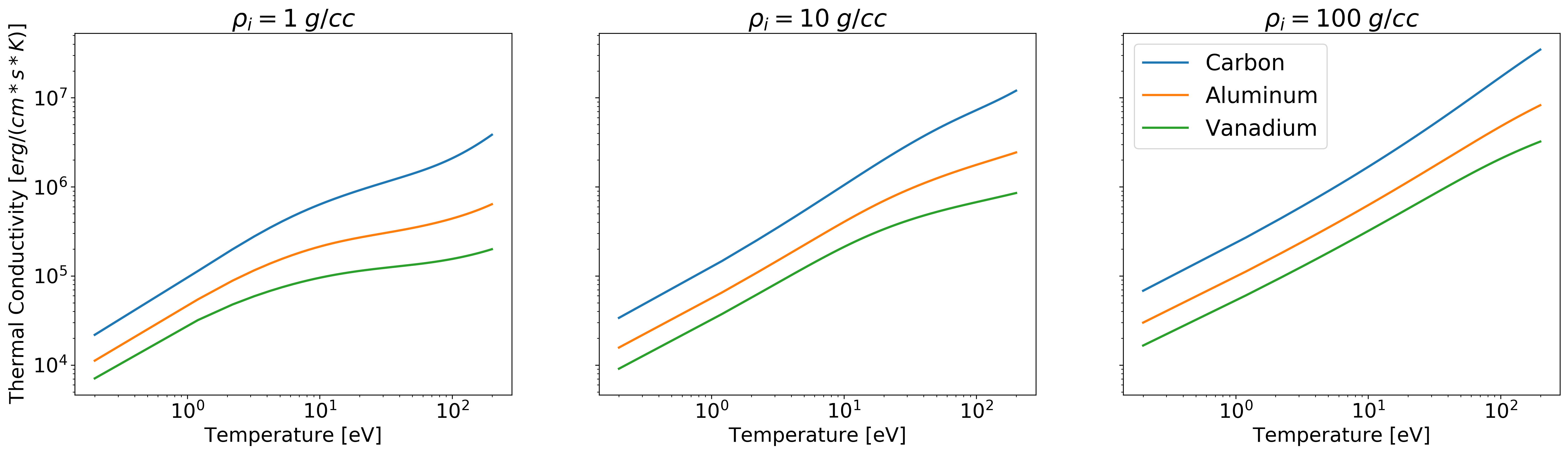
Example: Thermal Conductivity versus Temperature
import numpy as np
import matplotlib.pyplot as plt

from plasma_properties import transport

Am = np.array([1.9944235e-23, 4.4803895e-23, 8.4590343e-23]) # Atomic masses for each element (C, Al, and V) [g]
rho_i = np.array([1, 10, 100]) # Mass density range [g/cc]
T = np.arange(0.2, 200, 1) # Temperature range [eV]
Z = np.array([6, 13, 23]) # Nuclear charge of C, Al, and V

# Instantiate the Stanton-Murillo transport submodule
sm = transport.SM(Am, rho_i, T, Z, units_out='cgs')

# Compute Thermal Conductivity
K = sm.thermal_conductivity()

# Plotting
fig, ax = plt.subplots(1, 3, sharey=True, figsize=(24,6))

ax[0].loglog(T, K[0,:,0], linewidth=2)
ax[0].loglog(T, K[0,:,1], linewidth=2)
ax[0].loglog(T, K[0,:,2], linewidth=2)

ax[0].set_title('$\\rho_i = 1 \; g/cc$', fontsize=22)
ax[0].set_ylabel('Thermal Conductivity $[erg/(cm * s * K)]$', fontsize=18)
ax[0].set_xlabel('Temperature [eV]', fontsize=18)
ax[0].tick_params(axis="x", labelsize=18)
ax[0].tick_params(axis="y", labelsize=18)

ax[1].loglog(T, K[1,:,0], linewidth=2)
ax[1].loglog(T, K[1,:,1], linewidth=2)
ax[1].loglog(T, K[1,:,2], linewidth=2)

ax[1].set_title('$\\rho_i = 10 \; g/cc$', fontsize=22)
ax[1].set_xlabel('Temperature [eV]', fontsize=18)
ax[1].tick_params(axis="x", labelsize=18)
ax[1].tick_params(axis="y", labelsize=18)

ax[2].loglog(T, K[2,:,0], linewidth=2, label = 'Carbon')
ax[2].loglog(T, K[2,:,1], linewidth=2, label = 'Aluminum')
ax[2].loglog(T, K[2,:,2], linewidth=2, label = 'Vanadium')

ax[2].set_title('$\\rho_i = 100  \; g/cc$', fontsize=22)
ax[2].set_xlabel('Temperature [eV]', fontsize=18)
ax[2].tick_params(axis="x", labelsize=18)
ax[2].tick_params(axis="y", labelsize=18)

plt.legend(fontsize=20)
plt.show()
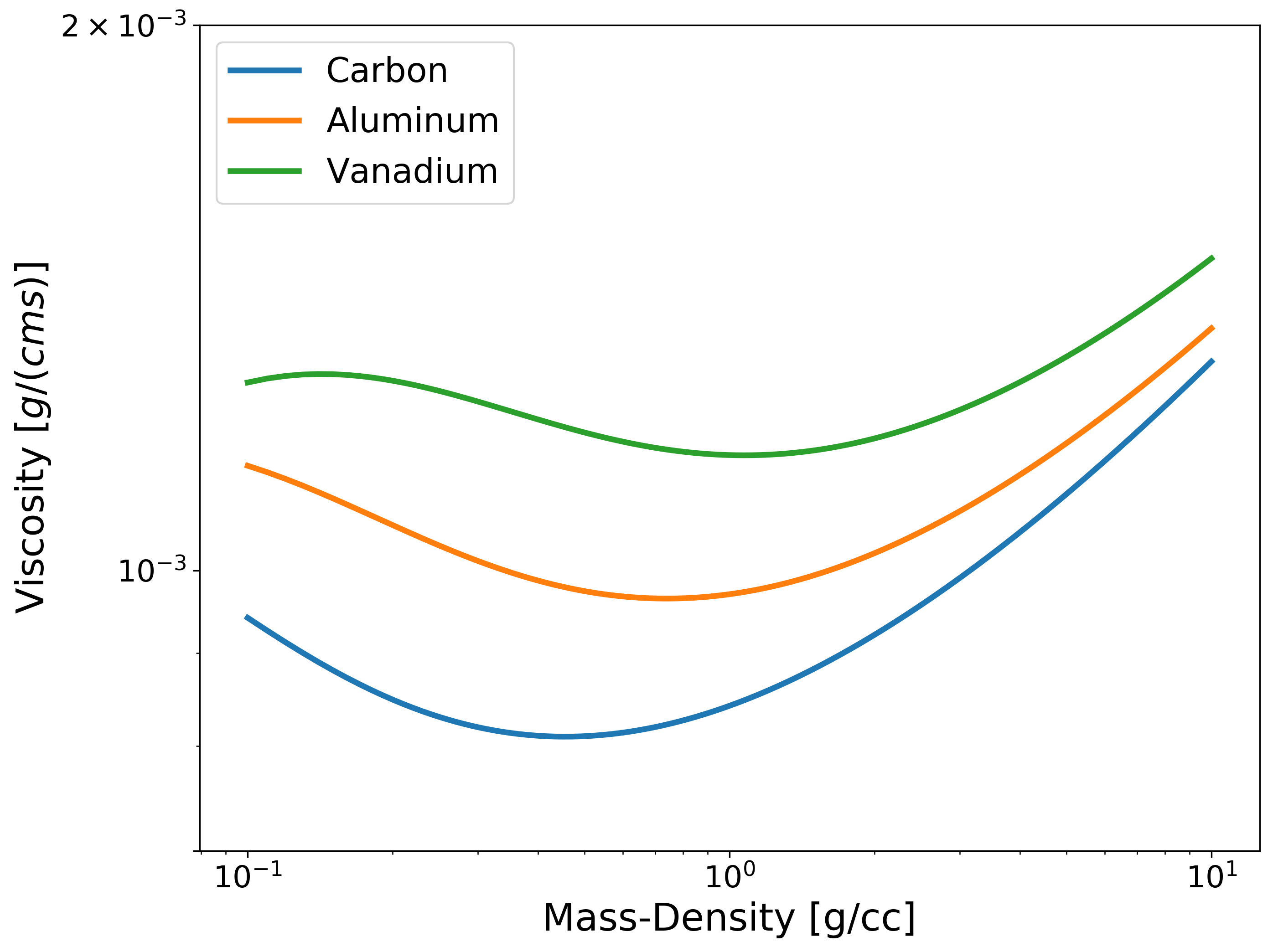
Example: Viscosity versus Density
import numpy as np
import matplotlib.pyplot as plt

from plasma_properties import transport

Am = np.array([1.9944235e-23, 4.4803895e-23, 8.4590343e-23]) # Atomic masses for each element [g]
rho_i = np.arange(0.1, 10, 0.01) # Mass densities [g/cc]
T = 0.2 # Temperature [eV]
Z = np.array([6, 13, 23]) # Nuclear charge for each element

# Instantiate the Stanton-Murillo transport submodule
sm = transport.SM(Am, rho_i, T, Z, units_out='cgs')

# Compute viscosity
eta = sm.viscosity()

# Plotting
plt.figure(figsize=(10,8))

# Plot viscosity versus density for fixed temp (0.1 eV)
plt.loglog(rho_i, eta[:,0,0], linewidth=3, label='Carbon')
plt.loglog(rho_i, eta[:,0,1], linewidth=3, label='Aluminum')
plt.loglog(rho_i, eta[:,0,2], linewidth=3, label='Vanadium')

plt.xlabel('Mass-Density [g/cc]', fontsize=20)
plt.ylabel('Viscosity $[g/(cm s)]$', fontsize=20)
plt.legend(fontsize=18, loc='upper left')
plt.yticks([7e-4, 1e-3, 2e-3])
plt.tick_params(axis="x", labelsize=16)
plt.tick_params(axis="y", labelsize=16)

plt.show()
Example: Transport for Different Isotopes and Elements
As mentioned in the note in the first section, the atomic mass and nuclear charge are coupled. To compute transport for different isotopes of the same element with additional elements, you will need to repeat the nuclear charge in the Z array but chance the atomic mass for each isotope. Fig. 2 shows a diagram of the data structure returned for the case of multiple isotopes and elements.
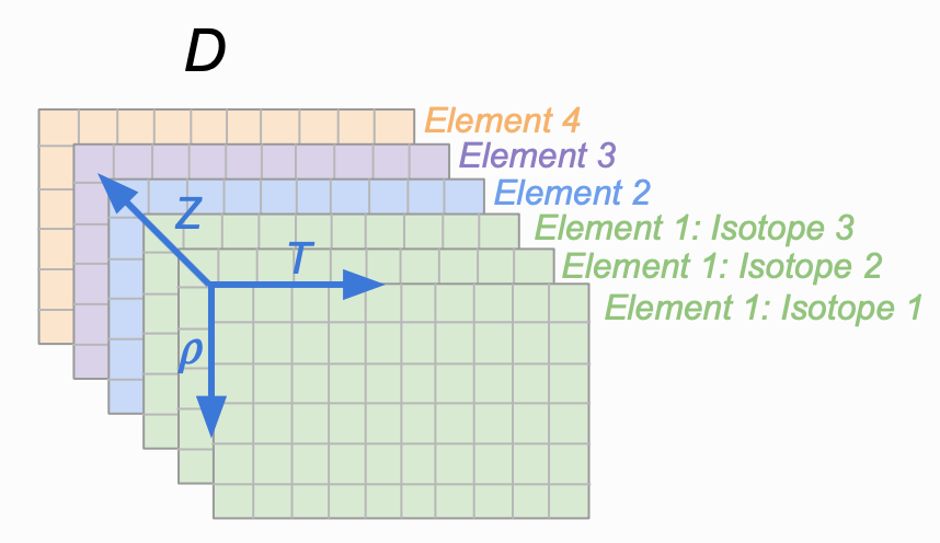
Fig 2. The shape of the data structure that is output for the case of multiple isotopes (each layer of green), and different elements (green, blue, purple, and orange layers).
import matplotlib.pyplot as plt
import numpy as np

from plasma_properties import transport

# Atomic mass [g] for each isotope/element - entries correspond to Z array
Am = np.array([1.6735575e-24, 3.344325e-24, 5.0082670843e-24, 1.1525801e-23, 1.9944235e-23, 4.4803895e-23])

# Mass density [g/cc]
rho_i = 1

# Temperature range [eV]
T = np.logspace(-1, 2, 20)

# Nuclear charge for each element - entries correspond to Am array
Z = np.array([1, 1, 1, 3, 6, 13])

# Create the stanton-murillo transport object
sm = transport.SM(Am, rho_i, T, Z, units_out='cgs')

# Compute self-diffusion
D = sm.self_diffusion()

# Plotting
cmap1 = plt.cm.get_cmap('Blues')
cmap2 = plt.cm.get_cmap('Set1')
plt.figure(figsize=(10,8))
plt.loglog(T, D[0,:,0], '-d', c=cmap1(125), linewidth=3, label='Hydrogen')
plt.loglog(T, D[0,:,1], '-v', c=cmap1(175), linewidth=3, label='Deuterium')
plt.loglog(T, D[0,:,2], '-x', c=cmap1(250), linewidth=3, label='Tritium')
plt.loglog(T, D[0,:,3], c=cmap2(0), linewidth=3, label='Lithium')
plt.loglog(T, D[0,:,4], c=cmap2(2), linewidth=3, label='Carbon')
plt.loglog(T, D[0,:,5], c=cmap2(3), linewidth=3, label='Aluminum')

plt.xticks(fontsize=16)
plt.yticks(fontsize=16)

plt.xlabel('Temperature [eV]', fontsize=18)
plt.ylabel('Self-Diffusion $[cm^2/s]$', fontsize=18)
plt.title('Self-Diffusion for Various Isotopes at $n_i = 10^{22} \; N/cc$', fontsize=18)
plt.legend(fontsize=18)

plt.show()
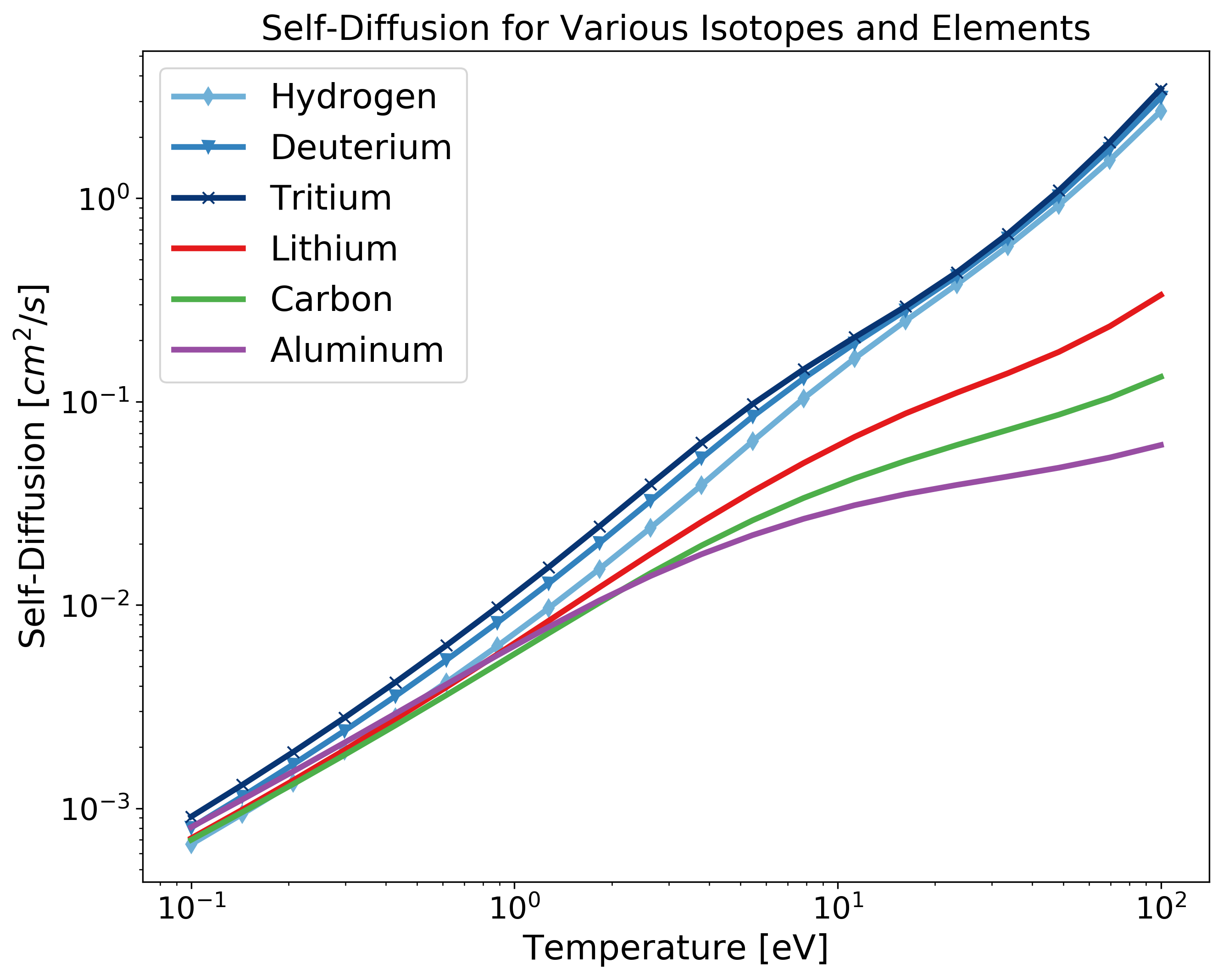
Fig 3. Note that the at first glance, the self-diffusion might be misleading for the above isotopes as hydrogen, a lighter element, diffuses less than tritium a heavier isotope. This is due to the fact that the mass density is kept constant for all atomic masses and the number density is computed inside the transport module. To make a comparison between isotopes/elements with the same number density see the next example.
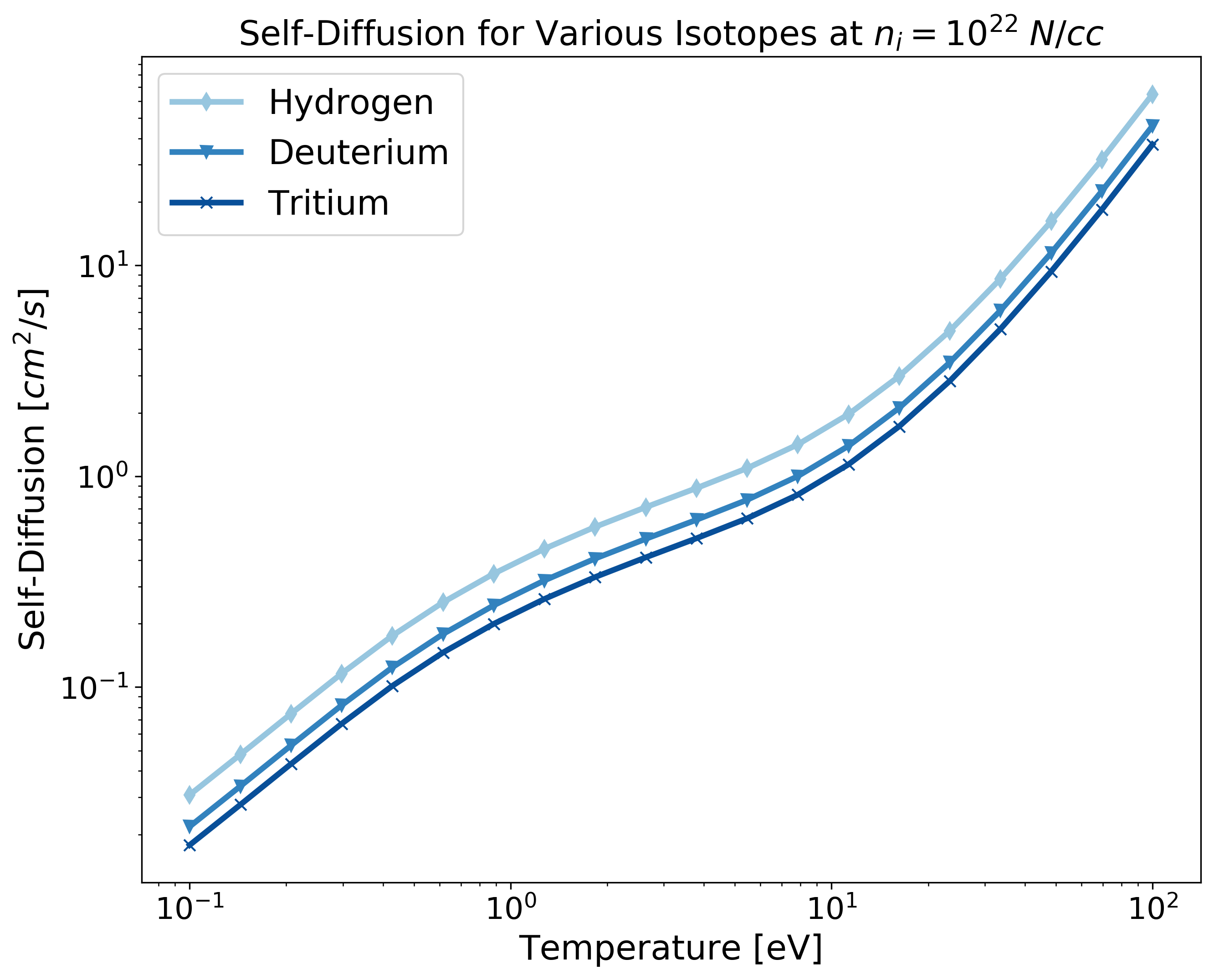
Example: Transport for Different Isotopes at Constant Number Density
import matplotlib.pyplot as plt
import numpy as np

from plasma_properties import transport

# Atomic mass [g] for each isotope/element - entries correspond to Z array
Am = np.array([1.6735575e-24, 3.344325e-24, 5.0082670843e-24])

# Specify number density
ni = 1e+22 # [N/cc]

# Compute the mass density needed for each isotope
rho_i = ni*Am

# Temperature range [eV]
T = np.logspace(-1, 2, 20)

# Nuclear charge for each element - entries correspond to Am array
Z = np.array([1,1,1])

# Create the stanton-murillo transport object
sm = transport.SM(Am, rho_i, T, Z, units_out='cgs')

# Compute self-diffusion
D = sm.self_diffusion()


# IMPORTANT: Note the array indexing in the following plotting command.
# To obtain the correct self-diffusion coefficient for the number density
# set above for each isotope, you must pick the the mass density index that
# corresponds to the isotope layer. For example, D[0,:,0] returns the
# self-diffusion coefficient across the temperature range for hydrogen with
# the ni set above. Similarly, D[1,:,1] returns the self-diffusion coefficient
# for deuterium at ni set above.

# Plotting
cmap = plt.cm.get_cmap('Blues')
plt.figure(figsize=(10,8))
plt.loglog(T, D[0,:,0], '-d', c=cmap(100), linewidth=3, label='Hydrogen')
plt.loglog(T, D[1,:,1], '-v', c=cmap(175), linewidth=3, label='Deuterium')
plt.loglog(T, D[2,:,2], '-x', c=cmap(225), linewidth=3, label='Tritium')

plt.xticks(fontsize=16)
plt.yticks(fontsize=16)

plt.xlabel('Temperature [eV]', fontsize=18)
plt.ylabel('Self-Diffusion $[cm^2/s]$', fontsize=18)
plt.title('Self-Diffusion for Various Isotopes at $n_i = 10^{22} \; N/cc$', fontsize=18)
plt.legend(fontsize=18)

plt.show()
Coming Soon!
Inter-diffusion
Electrical Conductivity
The Zbar Module
The current module for computing the mean ionization state (\(\langle Z \rangle\) or Zbar) is the Thomas-Fermi model (TF_Zbar). The returned data structure is the same structure as Fig. 1. Some example code and plots can be found below.
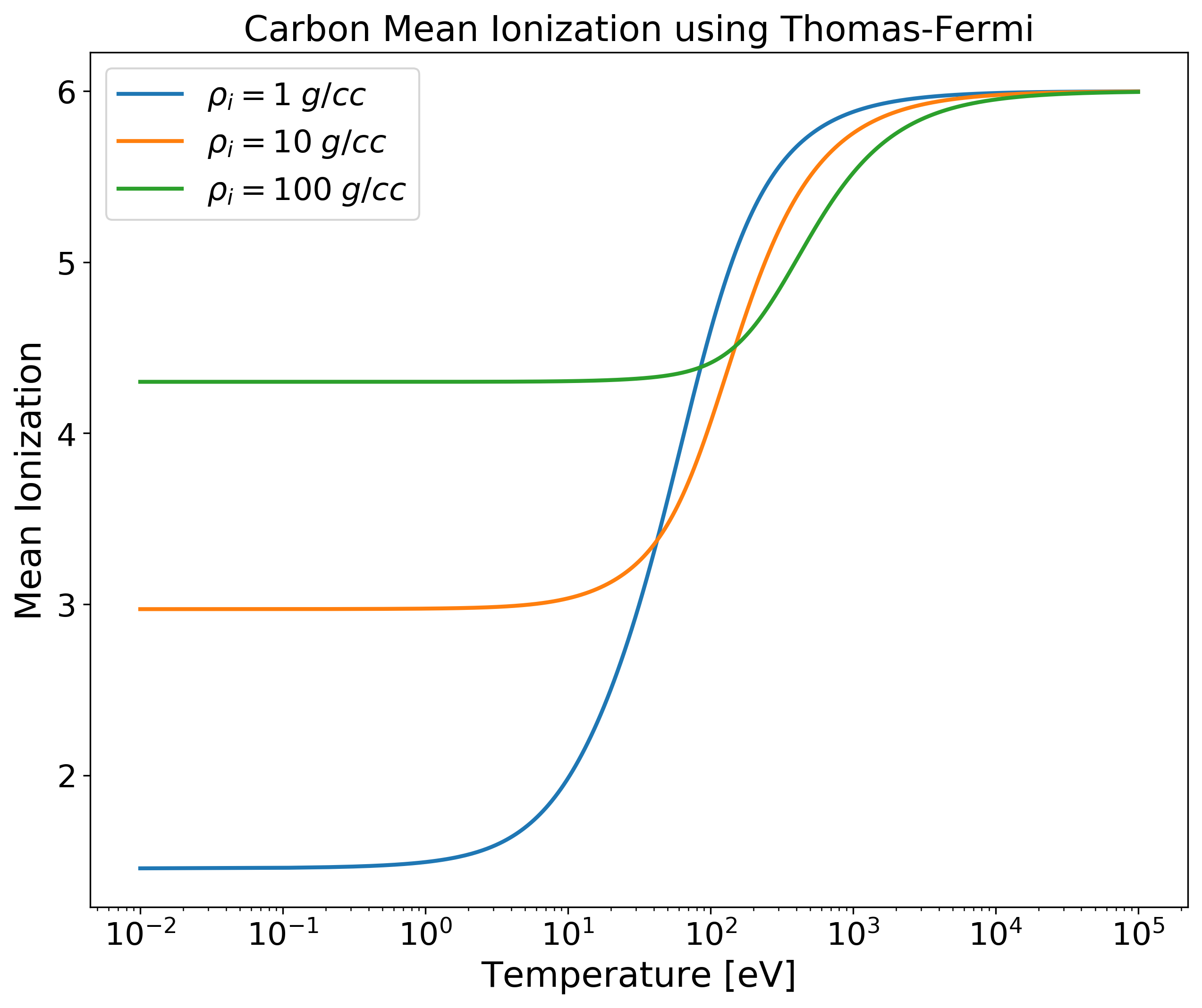
TF_Zbar for Single Element versus Temperature
import numpy as np
import matplotlib.pyplot as plt

from plasma_properties import zbar

# Initialize parameters for our system
Am = 1.9944235e-23 # Atomic mass [g]
rho_i = np.array([1, 10, 100]) # Mass densities [g/cc]
T = np.logspace(-2, 5, 100) # Temperature range [eV]
Z = 6 # Nuclear charge for carbon

# Create a mean ionization object
mi = zbar.MeanIonization(Am, rho_i, T, Z)

# Compute Thomas-Fermi zbar
Zbar = mi.tf_zbar()

# Plotting
plt.figure(figsize=(10,8))

# Plot each mass density for all temperatures for only the first element
plt.semilogx(T, Zbar[0,:,0], linewidth=2, label='$\\rho_i = 1 \; g/cc$')
plt.semilogx(T, Zbar[1,:,0], linewidth=2, label='$\\rho_i = 10 \; g/cc$')
plt.semilogx(T, Zbar[2,:,0], linewidth=2, label='$\\rho_i = 100 \; g/cc$')

plt.xticks(fontsize=16)
plt.yticks(fontsize=16)
plt.xlabel('Temperature [eV]', fontsize=18)
plt.ylabel('Mean Ionization', fontsize=18)
plt.title('Carbon Mean Ionization using Thomas-Fermi', fontsize=18)
plt.legend(fontsize=16, loc='upper left')

plt.show()
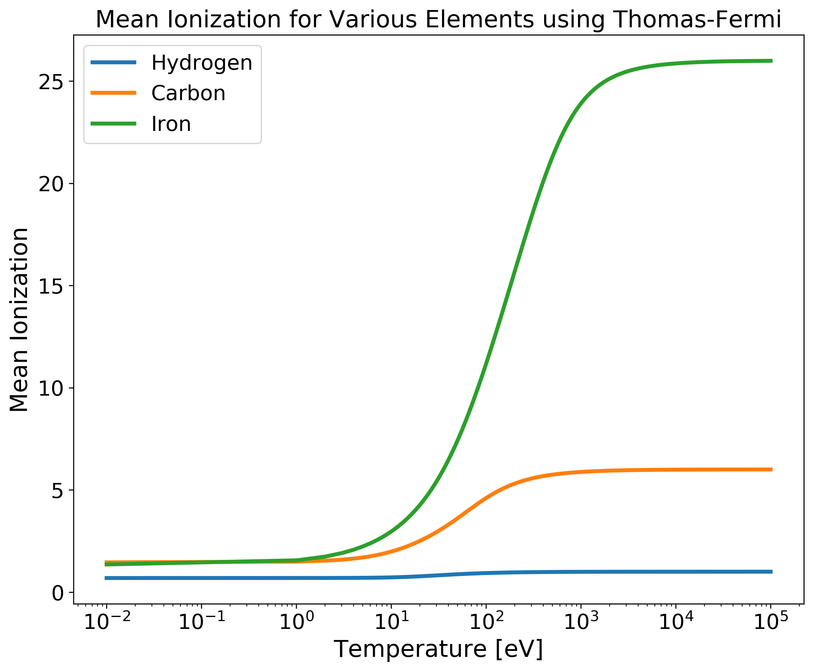
TF_Zbar for Multiple Elements versus Temperature
import numpy as np
import matplotlib.pyplot as plt

from plasma_properties import zbar

# Initalize parameters for our system
Am = np.array([1.6735575e-24, 1.9944235e-23, 9.2732796e-23]) # Atomic masses for each element [g]
rho_i = 1 # Mass densitiy for all elements [g/cc]
T = np.logspace(-2, 5, 100) # Temperature range [eV]
Z = np.array([1, 6, 26]) # Nuclear charge for each element

# Create a mean ionization object
mi = zbar.MeanIonization(Am, rho_i, T, Z)

# Compute Thomas-Fermi Zbar
Zbar = mi.tf_zbar()

# Plotting
plt.figure(figsize=(10,8))

plt.semilogx(T, Zbar[0,:,0], linewidth=2, label='Hydrogen')
plt.semilogx(T, Zbar[0,:,1], linewidth=2, label='Carbon')
plt.semilogx(T, Zbar[0,:,2], linewidth=2, label='Iron')

plt.xticks(fontsize=16)
plt.yticks(fontsize=16)

plt.xlabel('Temperature [eV]', fontsize=18)
plt.ylabel('Mean Ionization', fontsize=18)
plt.title('Mean Ionization for Various Elements using Thomas-Fermi', fontsize=18)
plt.legend(fontsize=16, loc ='upper left')

plt.show()
Coming Soon!
Saha Zbar
Multispecies Thomas Fermi Zbar
Hydrogenic Saha Zbar